Yvaine - Generative Animated SVG

February 08, 2025

Generative Animated SVG - Curve

Scroll Origins NFT

In 2023, Scroll launched the Scroll Origins NFT, and to date, 929,694 NFTs have bee‘n minted. You can view all of them on NFTScan. (V2)

nft-overview

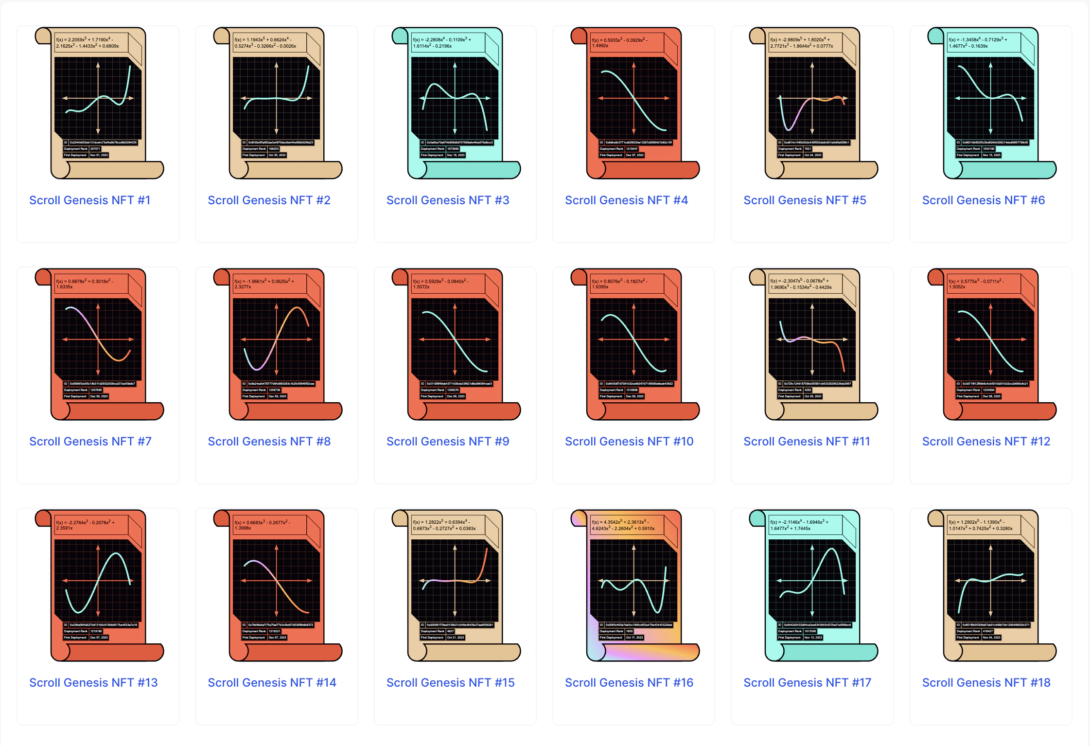
Overall, these NFTs are primarily divided into five styles:

Standard Styles:

Quintic function curve with a beige background
Quartic function curve with a cyan background
Cubic function curve with a rust background

Special Styles:

Any standard SVG with a rainbow curve
Any standard SVG with a rainbow background

Next, I’ll explain in detail how these NFTs (I mean, SVGs) are created. Let’s get started!

Background

One day, I received a SVG file from a discerning designer that looked incredibly scientific and elegant. I was told to generate various animated SVGs featuring different curves—each with four inflection points—while keeping the file size as small as possible, since the data needs to be stored on-chain.

After thoroughly analyzing the SVG source code, I optimized the SVG without compromising its rendering quality, slashing the file size from 138kb to just 7kb. In the progress, I also discovered that the curve consists of four segments of cubic Bézier curves. If we need to generate thousands of such curves, we must carefully choose functions to ensure the resulting curves remain both varied and elegant.

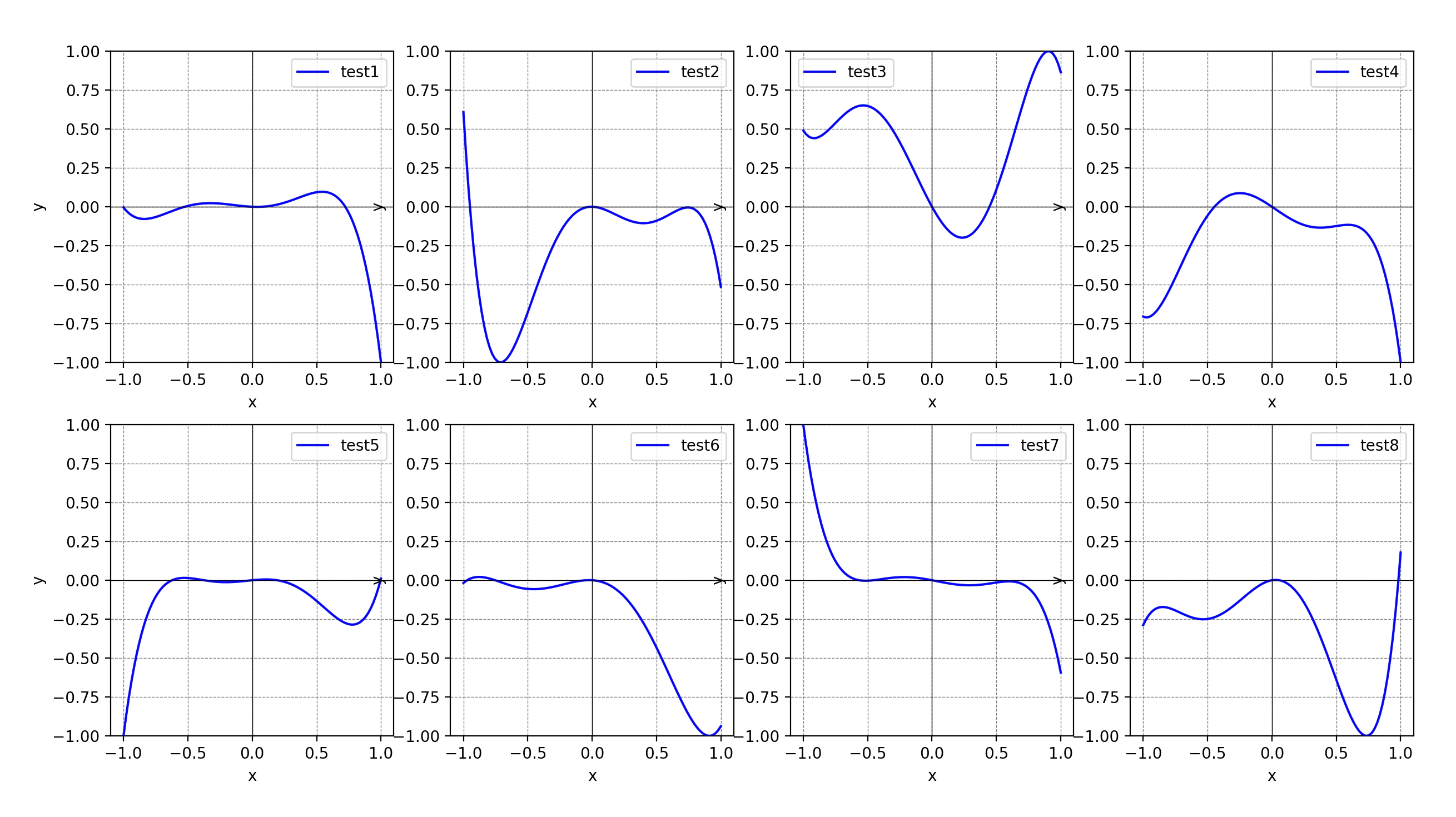
The next day, a brilliant researcher joined the channel and shared a Python file along with an amazing screenshot. py-5-degree He explained that the Python script generates high-order functions from random strings. Moreover, every curve it produces passes through the origin, with inflection points strictly confined to x ∈ [-1, 1] and y ∈ [-1, 1]. (So cool!)

Now, my first task is to generate three types of SVGs, each one showcases a curve generated by a cubic (with 2 inflection points), quartic (with 3 inflection points), or quintic (with 4 inflection points) function, paired with one of three background colors: beige, cyan, or rust. These will be distributed to users who deploy contracts on the Scroll Mainnet at different times.

I’m not a Python guy, but I’m a ChatGPT guy!

Well, let’s cook the SVG!

SVG Partitioning

First, segment the original SVG to isolate the sections that need to be generated programmatically. Then, annotate the code for each element group accordingly.

Clearly, this SVG comprises three dynamic regions:

Formula: Gererated from a random string
Curve on the coordinate axes: Derived by the formula
Descriptions: Displaying metadata

Accordingly, I added annotations to each region, and now everything appears neat and organized.

<!-- black bg -->
<g>
  <polygon
    class="st0"
    points="79.36,73.71 79.36,252.15 98.72,271.33 288.28,271.33 288.28,106.52 255.48,73.71"
  />
</g>
<!-- coordinate axes and arrows -->
<g>
  <polygon class="st7" points="183.82,85.77 179.15,98.58 188.49,98.58" />
  <polygon class="st7" points="183.82,259.27 188.49,246.46 179.15,246.46" />
  <line
    x1="183.82"
    y1="95.71"
    x2="183.82"
    y2="250.53"
    stroke="#EDCCA2"
    stroke-width="2"
  />
  ...
</g>
<!-- grid lines -->
<g>
  <line class="st6" x1="79.36" y1="85.77" x2="288.28" y2="85.77" />
  <line class="st6" x1="79.36" y1="103.12" x2="288.28" y2="103.12" />
  ...
</g>
<!-- formula -->
<text transform="matrix(1 0 0 1 83.8207 36.6262)"
  ><tspan x="0" y="0" class="st0 st83 st84">f(x)=4x^5+3x^4+2x^3</tspan
  ><tspan x="0" y="17.38" class="st0 st83 st84">+4x^2+6x+8</tspan></text
>

<!-- descriptions -->
<g>
  <rect x="98.72" y="300.06" class="st8" width="115.65" height="14.36" />
  <rect x="98.72" y="271.33" class="st8" width="16.36" height="14.36" />
  ...
</g>

<!-- curve -->
<path
  class="st61"
  d="M114.41,250.81c0,0,6.04-155.2,29.93 155.19c14.86,0.01,11.44,75.73,38.75,77.12s19.66,76.46,42.02,77.18 c27.47,0.89,28.13-155.26,28.13-155.26"
/>

Let’s begin by tackling the most challenging part: Curve.

Curve

Adjust the canvas

Before generating the curves programmatically, it’s crucial to define the canvas boundaries. The Python script outputs four inflection points (with x and y values within the [-1, 1] range) along with their corresponding formula from any given string. Therefore, we need a square canvas with the coordinate axes’ origin positioned at its center.

Next, I identified the coordinate axes background in the refined SVG, which was implemented using a <polygon>. In the original file, the Descriptions region masked the extra background at the bottom. So, I opted to use the top-right corner of the Descriptions region as the bottom-right corner of the coordinate axes background, thereby defining the area outlined by four red dots. Then, modified the polygon’s points to establish this new background.

After that, I analyzed the original grid lines and determined that each grid cell measures 17.35 units, with the origin at (183.82, 172.52). This allowed me to define a square canvas marked by four blue dots. With further calculations, I precisely positioned the grid lines, axes, and arrowheads.

All of this was done to ensure that every programmatically generated curve ultimately passes through the intersection of the coordinate axes on the static background.

Generate the path

There are two methods to generate the function curve:

Line Method (L Command)

Choose a sufficient number of points within the x-range of [-1, 1] and connect them sequentially with straight lines.

Pros
- Simple implementation by directly generating points based on the formula.
Cons
- If too few points are used, the resulting curve may appear jagged.
- Increasing the number of points for smoothness can significantly enlarge the SVG file size.
Curve Method (Q Command)

Select key points and generating the final curve using Bézier curves.

Pros
- Fewer key points are needed, keeping the SVG file size small.
- Ensures that the entire curve is smooth and follows a consistent arc.
Cons
- Some additional point coordinates must be computed as key points. For example, the function’s roots (where it intersects the x-axis).

After a quick test of connecting 100 points to generate the curve, the SVG size increased from 6,382 bytes to 9,963 bytes—an increase of over 1.5 times. Additionally, the inflection points exhibited noticeable jagged edges. appeared noticeably jagged. Consequently, I opted to use Bézier curves.

SVG supports two types of Bézier curves: quadratic and cubic. Ideally, cubic Bézier curves would better meet the requirements in both principle and effect. However, we currently only have the function formula and four inflection points. This means we also need to:

Compute the roots of the function
Compute the tangent line at each root
For each tangent line, select an appropriate point—either to the left or right—based on the extreme value’s position to create either a concave or convex arc.

Finding the Roots of a 5th-Degree Function

Since JavaScript doesn’t offer an efficient method for root finding, I turned to Python and used np.roots to obtain these coordinate.

import numpy as np
import sys
coefficientsStr = sys.argv[1]
coefficients = [float(x) for x in coefficientsStr.split(",")]
roots = np.roots(coefficients)
# Only the real roots are retained.
complex_indices = np.where(np.iscomplex(roots))
# Sort the real roots in ascending order based on their x-coordinates.
real_roots = np.array(sorted(np.real(x)
for x in np.delete(roots, complex_indices)))
rootsStr = ','.join(str(x) for x in real_roots)
print(rootsStr)

Then invoked it within NodeJS.

...
// Using Node’s execSync method to spawn a thread to run the Python script, which returns the x-coordinates of the multiple roots.
const xValues = execSync(`python ./findRoots.py ${formula.toString()}`);
const rootXValues = xValues.toString().split(",");
...

Plot Analysis

Now, we can generate the following plot. The meanings of the marked points are as follows:

The boundary points at x = -1 and x = 1
The roots, including the origin
The inflection points (local maxima or minima)

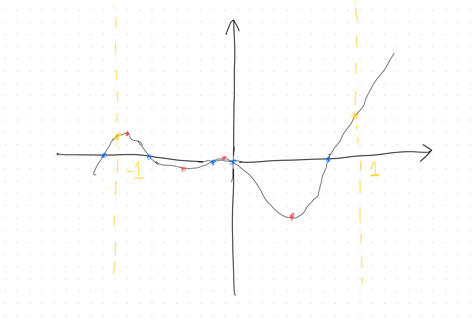
At this stage, rather than computing tangents at each root to construct cubic Bézier curves, the plot clearly shows that if we treat the blue/yellow points as endpoints and the red points as control points, the curve is roughly composed of four quadratic Bézier curves.

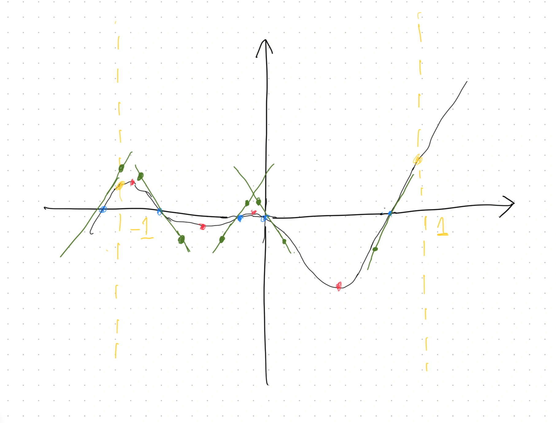
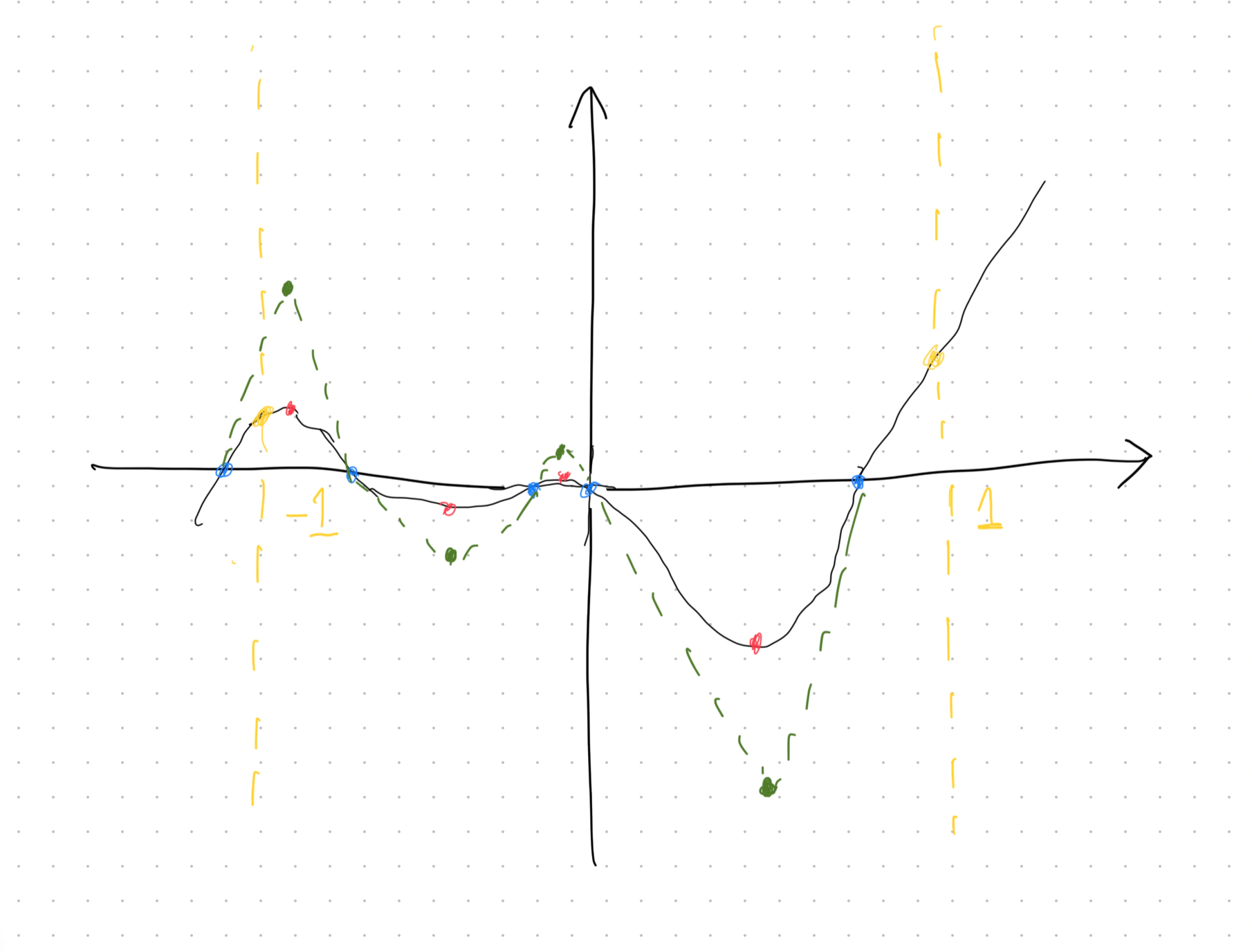
After adding the guide lines, the advantages of quadratic Bézier curves become clear:

There’s no need to compute the tangent for each root of an arbitrary fifth-degree function.
While cubic Bézier curves require eight control points (green dots), quadratic Bézier curves need only four. Moreover, the four control points can be scaled based on the Y-values of the inflection points.

At this point, I decided to use quadratic Bézier segments to generate the curve.

Selecting Key Points

In the ideal scenario, the function yields five roots, all with x-coordinates within [-1, 1]. When sorted in ascending order by x-coordinate, the key points are arranged as follows:

Boundary Point –Root – Inflection Point – Root – Inflection Point – Root – Inflection Point – Root – Inflection Point – Root – Boundary Point

This way, we can omit the blue boundary points. Amplifying the y-values of the inflection points yields the final set of path points:

Boundary Point – Amplified Inflection Point – Root – Amplified Inflection Point – Root – Amplified Inflection Point – Root – Amplified Inflection Point – Boundary Point

Accordingly, the SVG path value should be defined as:

M Boundary Point Q Amplified Inflection Point Root Q Amplified Inflection Point Root Q Amplified Inflection Point Root Q Amplified Inflection Point Boundary Point

However, things rarely work out perfectly, and several issues may arise:

If the leftmost root’s x-value is below -1, the key points don’t start with a boundary point. And similarly for the rightmost root.
A fifth-degree function may not yield five roots. In some cases, adjacent inflection points (red points) lack a root point(blue point), requiring an extra key point to be inserted between them (serving as a blue point, though marked green).
Although the extrema alternate between local maxima and minima, local minima aren’t always negative. This affects how we compute the enhanced red point. For instance, if a local minimum is negative, multiplying it by a factor greater than 1 makes it even smaller. If it’s positive, dividing by that factor achieves the desired amplification.

Therefore, when generating the path points using the key points, the following considerations must be taken into account:

The path points should always begin with the yellow point

Regardless of whether a root exists near the boundary, the boundary point always exists. Even if there’s a root to its left, using that root doesn’t guarantee the quadratic Bézier curve’s extrema will remain within the [-1, 1] range, visually resulting in a missing inflection point. Conversely, using the root to its right leads to an incomplete curve. Additionally, if the leftmost or rightmost root lies outside the [-1,1] range, using the boundary point yields a more pronounced curve.
When two adjacent points are yellow or blue, only one is retained

They serve as both the start or end points of the Bézier curve, so just one is sufficient.
Insert an extra auxiliary point between the two adjacent red points

If two red points appear consecutively, we need to compute an appropriate point between them as an endpoint. To simplify things and avoid extensive calculations, I selected the point with the median x-value to serve as the blue point.
Manually adjust the last point to be a yellow point

If the last collected point is blue, it should be replaced by the boundary point at x = 1 to ensure the curve remains intact.

const decidePathPoints = (allPoints) => {
  const result = [];
  let i = 0;
  while (allPoints[i].tag !== "yellow") {
    i++;
  }
  result.push(allPoints[i]);
  i += 1;
  for (let j = i; j < allPoints.length; j++) {
    if (
      ["yellow", "blue"].includes(allPoints[j - 1].tag) &&
      allPoints[j].tag === "red"
    ) {
      result.push(allPoints[j]);
    } else if (
      allPoints[j - 1].tag === "red" &&
      ["yellow", "blue"].includes(allPoints[j].tag)
    ) {
      result.push(allPoints[j]);
    } else if (
      allPoints[j - 1].tag === "yellow" &&
      allPoints[j].tag === "blue"
    ) {
      continue;
    } else if (allPoints[j - 1].tag === "red" && allPoints[j].tag === "red") {
      const x = calculateCenter(allPoints[j].x, allPoints[j - 1].x);
      const y = calculateCenter(allPoints[j].y, allPoints[j - 1].y);
      result.push({ x, y, tag: "green" }, allPoints[j]);
    }
  }
  if (result[result.length - 1].tag === "blue") {
    result.splice(result.length - 1, 1, allPoints[allPoints.length - 1]);
  }
  return result;
};

The key to generate amplified red points lies in:

Determine whether the current point is a local maximum or a local minimum.
Check if the computed y-value is positive or negative.
Decide whether to multiply by a factor or divide by it.

const maxViewportX = 153.62;
const maxViewportY = 153.62;

const embellishRedpoints = (formula, rootXValues, factor, tag) => {
  // Determine whether the original trend is upward or downward based on the first two extrema.
  const trend = Math.sign(rootXValues[1] - rootXValues[0]);
  return rootXValues.map((item, index) => {
    // calculate the Y-value based on the formula.
    const y = calculateYFromFormulaAndX(formula, item);
    // Since local maxima and minima always alternate, you can determine whether the current point is a maximum or a minimum accordingly.
    const isMaximum = (index % 2 === 0 ? 0 : 1) & (trend === 1 ? 1 : 0);
    let enhancedY;
    if (isMaximum) {
      if (y > 0) {
        enhancedY = y * factor;
      } else {
        enhancedY = y / factor;
      }
    } else {
      if (y < 0) {
        enhancedY = y * factor;
      } else {
        enhancedY = y / factor;
      }
    }
    return {
      // Will explain in next section
      x: +transX(item, maxViewportX).toFixed(4),
      y: +transY(enhancedY, maxViewportY).toFixed(4),
      tag,
    };
  });
};

Coordinate System Transformation

In a mathematical coordinate system, the origin is at the center. However, in the SVG coordinate system, the origin is located at the top-left corner.

This requires converting and scaling the point coordinates so they align perfectly within the square canvas defined by the four blue dots. In practice, to maintain a margin from the sharp tips of the axis arrowheads, I opted for a slightly smaller canvas than the full square.

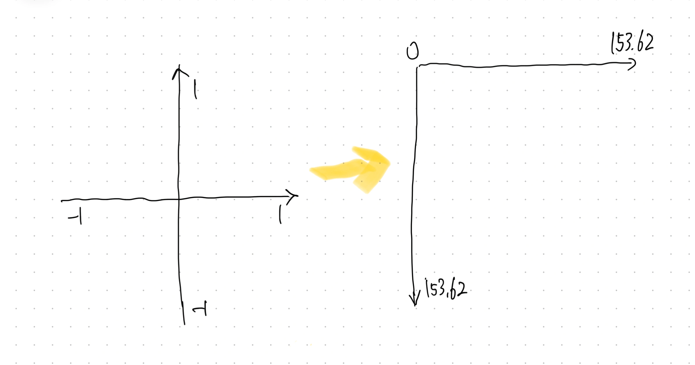
For the final canvas, which measures 153.62 x 153.62, I mark the top-left corner at (107.01, 95.71). By applying a <g> element’s transform attribute, I set this point as the origin of the SVG coordinate system for the curve. This adjustment simplifies subsequent calculations, as starting from (0, 0) is much easier than starting from (107.01, 95.71).

const maxViewportX = 153.62;
const transX = (value, maxViewportX) => {
  const dd = maxViewportX / 2;
  if (value < 0) {
    // Note that the amplifying for positive and negative values is reversed
    return dd - dd * Math.abs(value);
  }
  return dd + dd * value;
};
// The same applies to the Y values

Code

Ultimately, the code for the curve looks like below:

<g transform="translate(107.01, 95.71)">
  <path
    class="curve"
    d="M0 58.9594 Q5.1475 43.8068, 19.0479 76.8075 Q46.0658 140.8778, 76.81 76.81 Q95.4768 46.615, 112.0631 76.8113 Q141.2229 184.3478, 153.62 107.3804"
  />
</g>

Animate the Path

For <path>, the stroke attribute defines the line of the shape. Two properties related to stroke are particularly useful for animations:

stroke-dasharray

This property defines a dash pattern along the path. For example, setting stroke-dasharray: 1000; creates an alternating pattern of 1000 units of drawn line followed by 1000 units of gap. If the actual length of the path is less than 1000, the entire path appears as a solid line.
stroke-dashoffset

This property specifies the starting offset of the dash pattern. For example, with stroke-dasharray: 1000; and stroke-dashoffset: 800;, the drawing skips the first 800 units of the path, then renders 200 units of solid line before continuing with the dash pattern.

By these two properties, can create dynamic stroke animations along the path.

.path {
  /* For convenience, I uniformly set the value to 1000, since I’m confident that the path length will not exceed 1000. */
  stroke-dasharray: 1000;
  /* Each animation loops every 3 seconds, with a 4ms gap between cycles */
  /* In reality, the effective interval between animations is greater than 4ms */
  /* Since the path is definitely shorter than 1000 units, part of the 3-second duration is essentially “wasted” on the dash offset corresponding to the difference between 1000 and the actual path length */
  animation: draw 3s linear 4ms infinite;
}

/* 1000->0 the line gradually emerges from 0 length to full length */
@keyframes draw {
  from {
    stroke-dashoffset: 1000;
  }

  to {
    stroke-dashoffset: 0;
  }
}

Show the final Curve

Tada! We’ve generated a curve with four inflection points that passes through the origin and features an animation where the line draws itself repeatedly from left to right. Moreover, each random string produces a unique curve. While some root transitions may be a bit awkward, the smooth arcs instead of jagged edges create a visually pleasing, rounded effect.

What's the next?

Once the most challenging part is behind us, everything else becomes much simpler. The same approach applies to both quartic functions with three inflection points and cubic functions with two inflection points.

With that foundation in place, we can confidently proceed to render Formula & Descriptions.